
MINIST
MNIST 데이터셋은 손으로 쓴 숫자(0에서 9까지) 이미지로 이루어진 대표적인 머신러닝 데이터셋 중 하나이다. 이 데이터셋은 기계 학습과 딥 러닝 모델의 기본적인 벤치마크로 사용되며, 숫자를 인식하는 모델을 훈련하고 평가하는 데에 널리 활용된다.
설정
from tensorflow.keras.models import Sequential
from tensorflow.keras.layers import Dense, Activation
from tensorflow.keras.utils import to_categorical
from tensorflow.keras.datasets import mnist
import numpy as np
import matplotlib.pyplot as pltTensor Flow 및 관련 라이브러리를 불러왔다. 이러한 라이브러리를 사용하여 MNIST 데이터셋을 불러오고 모델을 구축하며, 결과를 시각화하는 과정을 진행할 것이다.
# MNIST 데이터셋 로드
(x_train, y_train), (x_test, y_test) = mnist.load_data()

# 데이터 형태 출력
print("X_train shape", x_train.shape)
print("y_train shape", y_train.shape)
print("X_test shape", x_test.shape)
print("y_test shape", y_test.shape)
MNIST 데이터셋은 훈련 데이터 (x_train, y_train)와 테스트 데이터 (x_test, y_test)로 나뉜다. 각 데이터의 형태를 출력해 보면 훈련 이미지는 28x28 픽셀의 2D 배열로 이루어져 있으며, 훈련 레이블은 숫자의 정수값으로 표현된다. 훈련 데이터는 60,000개의 샘플로 구성되어 있고, 테스트 데이터는 10,000개의 샘플로 구성되어 있음을 확인할 수 있다.
데이터 전처리
데이터를 전처리하는 것은 모델이 데이터를 이해하고 효과적으로 학습할 수 있도록 데이터를 변환하는 과정이다.
먼저, 이미지 데이터를 신경망에 입력하기 적합한 형태로 변환해야 한다. MNIST 이미지는 28x28 픽셀의 2D 배열로 구성되어 있지만, 이를 신경망에 입력하기 위해서는 1D 벡터로 평탄화(flatten)해야된다. 또한, 입력 데이터의 값 범위를 0에서 1 사이로 스케일링해 주었다.
# 이미지 데이터 전처리
X_train = x_train.reshape(60000, 784)
X_test = x_test.reshape(10000, 784)
X_train = X_train.astype('float32')
X_test = X_test.astype('float32')
X_train /= 255
X_test /= 255

# 전처리된 데이터 형태 출력
print("X Training matrix shape", X_train.shape)
print("X Testing matrix shape", X_test.shape)먼저 reshape 메서드를 사용하여 이미지 데이터를 1차원 벡터로 변환하고, 데이터 타입을 float32로 변경하였다. 그리고 각 픽셀 값(0에서 255)을 0과 1 사이의 값으로 스케일링을 진행해 주었다.
레이블 전처리
# 레이블 전처리
nb_classes = 10
Y_train = to_categorical(y_train, nb_classes)
Y_test = to_categorical(y_test, nb_classes)

# 전처리된 레이블 형태 출력
print("Y Training matrix shape", Y_train.shape)
print("Y Testing matrix shape", Y_test.shape)레이블을 원-핫 인코딩 형태로 변경하기 위해 to_categorical 함수를 사용해주었다.
모델 생성 및 컴파일
# 모델 생성
model = Sequential()
model.add(Dense(512, input_shape=(784,)))
model.add(Activation('relu'))
model.add(Dense(256))
model.add(Activation('relu'))
model.add(Dense(10))
model.add(Activation('softmax'))

# 모델 요약 정보 출력
model.summary()

# 모델 컴파일
model.compile(loss='categorical_crossentropy', optimizer='adam', metrics=['accuracy'])

# 모델 훈련
model.fit(X_train, Y_train, batch_size=128, epochs=50, verbose=1)'categorical_crossentropy' 손실 함수와 'adam' 옵티마이저를 사용하여 모델을 컴파일하였으며, 정확도(metrics)를 기록합니다. 모델은 훈련 데이터를 이용하여 50 에포크 동안 훈련됩니다.
학습 결과
# 학습 결과 및 시각화
score = model.evaluate(X_test, Y_test)
print('Test score:', score[0])
print('Test accuracy:', score[1])
predicted_classes = np.argmax(model.predict(X_test), axis=1)
correct_indices = np.nonzero(predicted_classes == y_test)[0]
incorrect_indices = np.nonzero(predicted_classes != y_test)[0]
plt.figure()
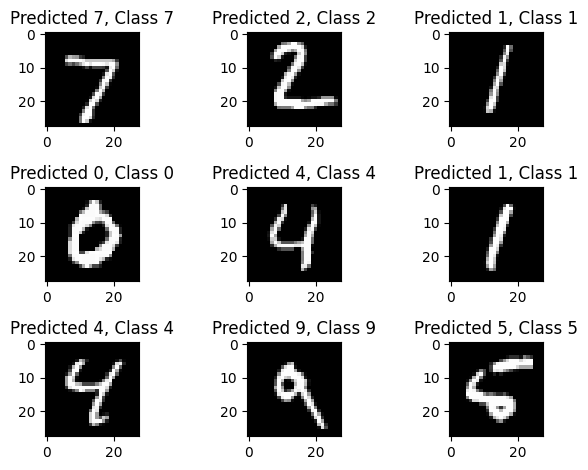
# 정답 예측 이미지 시각화
for i, correct in enumerate(correct_indices[:9]):
plt.subplot(3,3,i+1)
plt.imshow(X_test[correct].reshape(28,28), cmap='gray', interpolation='none')
plt.title("Predicted {}, Class {}".format(predicted_classes[correct], y_test[correct]))
plt.tight_layout()
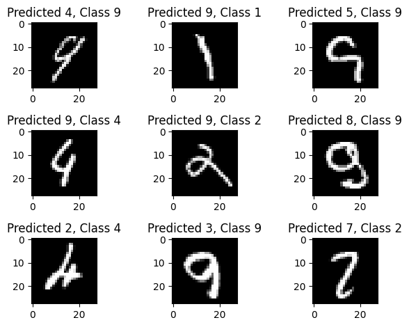
# 오답 예측 이미지 시각화
plt.figure()
for i, incorrect in enumerate(incorrect_indices[:9]):
plt.subplot(3,3,i+1)
plt.imshow(X_test[incorrect].reshape(28,28), cmap='gray', interpolation='none')
plt.title("Predicted {}, Class {}".format(predicted_classes[incorrect], y_test[incorrect]))
plt.tight_layout()모델을 테스트 데이터로 평가하고, 테스트 손실과 정확도를 출력하며, 정확하게 예측한 이미지와 오답 예측한 이미지를 시각화한다.
# 테스트 손실: 0.13196906447410583
# 테스트 정확도: 0.98089998960495내 손글씨 숫자 예측하기
이제 모델을 사용하여 직접 그린 손글씨 숫자를 예측하려고 한다. 아래 코드는 내 손글씨 이미지를 모델에 입력하고 예측하는 과정이다.
import cv2
import numpy as np

# 이미지 로드 및 전처리
image_path = 'your_image.jpg'  # 이미지 파일 경로 설정
image = cv2.imread(image_path, cv2.IMREAD_GRAYSCALE)
image = cv2.resize(image, (28, 28))
image = image.astype('float32') / 255.0
image = image.reshape(1, 784)  # 모델이 기대하는 형태로 변환

# 이미지 예측
predictions = model.predict(image)

# 예측 결과 확인
predicted_class = np.argmax(predictions)
print("Predicted class:", predicted_class)
1/1 [==============================] - 0s 38ms/step
Predicted class: 7
1/1 [==============================] - 0s 22ms/step
Predicted class: 5위 코드를 실행하면 모델이 입력된 손글씨 이미지를 분석하고 예측된 숫자를 출력한다. 그려진 숫자와 모델의 예측 결과를 비교하여 모델의 성능을 확인할 수 있는데, 모델의 설계 당시 98점의 높은 점수를 보여주었으나, 2를 7이라고 예측하는 모습을 보여준다.
결론
결론 이 글에서는 MNIST 데이터셋을 사용하여 숫자 인식 모델을 구축하고 훈련하는 방법을 알아보았다. 또한, 해당 모델을 직접 그린 손글씨 숫자에 대한 예측에 적용하고 모델의 성능을 확인해 보았다. 모델은 설계 당시 높은 정확도를 보였지만, 일부 경우에는 예측이 정확하지 않을 수 있음을 확인할 수 있었다.
해당 내용은 김성규 교수님의 수업을 바탕으로 정리하였습니다.